Phys 198                                     January 27, 1997

PHOTOELASTICITY

Elasticity: Strain and Stress

Strain: Measure the distance L_o between two points on the surface of a specimen and apply some form of loading (e.g. mechanical, thermal). This will cause deformation of the specimen, and the distance between the two points will change. The strain e is the ratio of the change in length to the original length: .e = DL/L_o = (L' - L_o)/L_o. Note that strain is dimensionless; also, since the change in length of many materials (e.g., metals) is usually quite small for normal loads, strain is frequently expressed in units of microstrain me where the numerical value given has been divided by 10 ^-6. If the traditional cartesian coordinate system (x,y,z) is used and the displacement along each axis is measured as (u,v,w), then certain standard units can be used. For instance, if the strain at a surface can be projected onto the normal to the surface, the strain can be expressed in terms of a normal strain component perpendicular to the surface and of two shearing strain components parallel to the surface. These directions are called principal axes and the strain components are called the principal strain components. If a small cube is taken around a point, it is seen that there are three principal axes orthonormal to each other. Using one subscript to describe the principal axis involved and a second subscript to describe the direction of the strain component, a three-by-three matrix is obtained describing the strain at that point. For instance, considering the surface normal pointing in the x direction, the strain components can be described by e_xx, g_xy,g_xz..Using the definition of strain given above, the strain components are

• e_xx = DL_x/L_ox = (L'_x - L_ox)/L_ox = du/dx
• g_xy = du/dy + dv/dx
• g_xz = dw/dx + du/dz

Stress: When a force F is applied to a body, its effect is felt throughout the body. At any selected point in the body, the stress t at that point is defined as the net force acting there divided by a small area DA in a plane containing the point and normal to the force at that point in the limit as DA goes to zero: t = F/dA . Using standard projection techniques, the components (s₁, s₂, s₃) of the stress t along a specified cartesian coordinate system at the selected point can be determined. Generally the interest is in stresses at the surface of a body and particularly the stress as expressed in components perpendicular to and parallel to the body surface. When the stress vector is broken down into such components, the results are called the principal stress components. These are usually ranked in order of decreasing magnitude and referred to as s₁ >= s₂ >= s₃.

Note: Detailed information on stress and strain can be found in standard texts, e.g., Dally and Riley, Experimental Stress Analysis, Third Edition, McGraw Hill, 1991. Chapters 1 and 2.

Photoelastic Studies:

In photoelastic studies, most work is done measuring two-dimensional stress using plane models. In this case, there are only the two in-plane components s_x and s_y, usually designated as s₁ and s₂. Note that in this case there is no claim that s₁ > s₂. The materials used for making models in photoelastic studies (various types of plastics, acrylics, Lucite, etc.) are birefringent. In addition, the amount of birefringence (n₁ - n₂) varies linearly with the forces applied and thus with the stress at any point. This birefringent effect is due to the changes in molecular spacing which result from the applied forces, and is discussed in solid state texts or books on the strength of materials. However, as our textbook author points out, it is still not fully understood. Since the plastic models are flat sheets, the thickness t of the material is everywhere the same. Only a biaxial stress is involved and the two indicies of refraction due to birefringence are proportional to this biaxial stress (n_i = C_is_i, i = 1,2). It can be shown that the linear relation between n_i and s_i can be expressed in two linear equations R₁ = (C₁s₁ + C₂s₂)t and R₂ = (C₂s₁ + C₁s₂)t which after some math leads to R = C(s₁ - s₂)t, where C is the stress-optic coefficient of the material, so the relative retardation R = (n₁ - n₂)t = C(s₁- s₂)t depends linearly on the amount of stress. This leads to the result that as the stress varies, the birefringence will vary, and the retardation will vary. Therefore the color extinction effect will act on different wavelengths as the stress changes and a stress field will appear as a set of colored bands which correspond to the varying stress over the field. Such bands are called isochromatics. Of course the color of the band is not that of the extinguished color, but rather that of its complement. While in fact these bands do not give the value of the two principal stresses separately, but only their difference (s₁ - s₂), it can be shown that this difference is equal to twice the maximum shear stress at this point, i.e., (s₁ - s₂) = 2t_max, which is frequently sufficient information for the purposes of the study. Since C is material specific and geometry independent, the thickness t of the two-dimensional plate must be taken into account, and the maximum shear stress value obtained by counting fringes is given by t = CN/(2t), where N is the fringe count. At locations of uniaxial stress (free boundaries), the value of the complete stress is determinable. In general, the ability to separate the two stress components requires additional measurements. Consider also that if the birefringent effect is viewed through crossed polarizers, and the principal axes of the refractive indicies (n₁ and n₂) are aligned with the polarization axes, no light will get through the system and a black line will connect those spots at which these axes are aligned. These black lines are called isoclinics because they indicate the inclination or angle of the stress vector with respect to the analyzer. These lines are used to determine the orientation of the stress vector at any point. Thus both the orientation and the magnitude of the maximum shear stress vector at any point can be determined by studying the isoclinics and the isochromatics.

Note: All of this material on photoelasticity is explained in depth in the course testbook, Chapter 4.

Color

The following image shows the resulting colors when primary colors are combined. The image is meant to be helpful, but the quality of reproduction limits the accuracy of the color shadings.

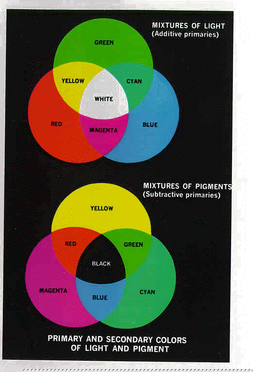
Color Representations and Models:

• RGB - Color Cube (used for video displays)
  Red, Green, and Blue are the primary colors here , with the secondary colors Cyan, Magenta, and Yellow (CMY) as their respective complementary colors, and are used in an additive mode such that equal amounts of all three will produce White. In the color cube model, each corner of a unit cube is defined as one of the primary or secondary colors. The primary axes are labelled Red, Green, and Blue, with the origin (0,0,0) black, and the maximum corner (1,1,1) is white. Any spot in the cube is a color represented by the value of the three primary colors.
• CMYK - Color Cube (used for printing)
  Cyan, Magenta, and Yellow are the primary colors here, with the secondary colors RGB being their respective complementary colors. These are colors used subtractively, such that equal amounts of all three will produce Black. Actually, in the real world of printing dyes, these three colors do not produce a good black, so a fourth basic color Black (K) is added to the list of primaries.
• HSI - Color Pyramid or Cone (used in image processing)
  Hue, Saturation, and Intensity are the basic characteristics here. Hue gives the basic color, Saturation gives how intense the color is, or alternatively, how much white is added to the Hue. Red with low saturation would be pink, while Red with high saturation would be bright scarlet. Intensity gives the total illumance present; if the intensity is low, the picture is very dark, while a high Intensity means the picture is bright. In the HSI model, Hue is the amount of angular rotation around the z-axis, measured from the x-axis, Saturation is the radial distance from the center, with the saturation increasing with distance from the centerThe advantage of the HSI model over say the RGB model, is that changing these parameters in an image produces changes that correspond to the user's expectation. This model is widely used in interactive image editing.
• YIQ - Transmission system used for Color Television signals
  Y is illuminance, while I (In-Phase) and Q (Quadrature Phase) are chrominance. This system is used in the TV industry, because it allows ordinary black-and-white TV sets to pick up a color picture by just using the illumance Y, which is essentially the gray scale version of the image. I and Q are controlled by varying their phase with respect to the illuminance so as to send information about colors. In a color TV set, these three data signals (YIQ) are converted to RGB and then displayed on the TV monitor.

Additive and Subtractive Primaries:

• Primaries
• Secondaries

Complementary Colors

Note: A detailed discussion of these aspects of color can be found in Gonzalez & Woods, Digital Image Processing, Addison-Wesley, 1993. Chapter 4, Section 4.6.